Example usage
In this notebook, I will demonstrate how to use msions to create MS TIC and ion plots.
Imports
import msions.mzml as mzml
import msions.hardklor as hk
import msions.percolator as perc
import msions.kronik as kro
import msions.msplot as msplot
import msions.encyclopedia as encyclo
import msions.utils as msutils
import matplotlib.pyplot as plt
Create DataFrame from mzML file
tic_df creates a pandas DataFrame of MS1 scan information from an mzML file.
ms1_df = mzml.tic_df("example_files/DIA_file.mzML")
It can also be used to make a DataFrame of MS2 scan information
ms2_df = mzml.tic_df("example_files/DDA_file.mzML", level="2")
or a DataFrame with both sets of information.
ms_df = mzml.tic_df("example_files/short_DDA_file.mzML", level="all", include_ms1_info=True)
peak_df creates a pandas DataFrame containing the m/z, ion current, and retention time for all MS1 peaks.
ms1_peaks = mzml.peak_df("example_files/short_DDA_file.mzML")
Read Hardklor file
hk2df will read a Hardklor tab-delimited file into a pandas DataFrame. After import, all columns that can be converted to a numeric data type will be.
hk_df = hk.hk2df("example_files/DIA_hk.hk")
summarize_df will summarize the TIC in each scan from a Hardklor pandas DataFrame or Hardklor tab-delimited file.
hk.summarize_df(hk_df)
| rt | scan_num | TIC | |
|---|---|---|---|
| 0 | 0.0051 | 1 | 14409796 |
| 1 | 0.0574 | 152 | 15346213 |
| 2 | 0.1091 | 303 | 16216937 |
| 3 | 0.1607 | 454 | 16422145 |
| 4 | 0.2124 | 605 | 15524068 |
| ... | ... | ... | ... |
| 2493 | 99.9866 | 291311 | 108058 |
| 2494 | 99.9897 | 291312 | 24495 |
| 2495 | 99.9927 | 291313 | 51831 |
| 2496 | 99.9958 | 291314 | 424145 |
| 2497 | 99.9989 | 291315 | 111484 |
2498 rows × 3 columns
If an additional pandas DataFrame is provided with the MS1 scan information, the ion injection time will be mapped to each scan.
hk.summarize_df(hk_df, ms1_df)
| scan_num | rt | TIC | IT | ions | |
|---|---|---|---|---|---|
| 0 | 1 | 0.0051 | 14409796.0 | 50.000000 | 720489.800000 |
| 1 | 152 | 0.0574 | 15346213.0 | 40.343060 | 619113.184769 |
| 2 | 303 | 0.1091 | 16216937.0 | 40.586967 | 658196.294454 |
| 3 | 454 | 0.1607 | 16422145.0 | 43.578297 | 715649.106626 |
| 4 | 605 | 0.2124 | 15524068.0 | 40.905605 | 635021.398509 |
| ... | ... | ... | ... | ... | ... |
| 2560 | 291311 | 99.9866 | 108058.0 | 50.000000 | 5402.900000 |
| 2561 | 291312 | 99.9897 | 24495.0 | 50.000000 | 1224.750000 |
| 2562 | 291313 | 99.9927 | 51831.0 | 50.000000 | 2591.550000 |
| 2563 | 291314 | 99.9958 | 424145.0 | 50.000000 | 21207.250000 |
| 2564 | 291315 | 99.9989 | 111484.0 | 50.000000 | 5574.200000 |
2565 rows × 5 columns
Create a simplified DataFrame from a Kronik file
simple_df can be used to filter a Kronik DataFrame’s rows and columns.
kro_df = kro.simple_df("example_files/DDA_match.kro")
filter_df can be used to filter a Kronik DataFrame within a retention time range.
kro.filter_df(kro_df, start=20, stop=80)
| first_scan | last_scan | num_scans | mass | charge | best_int | sum_int | best_rt | mz | best_rt_s | |
|---|---|---|---|---|---|---|---|---|---|---|
| 0 | 38596 | 44919 | 225 | 841.5023 | 2 | 1.483303e+10 | 5.915766e+11 | 24.8667 | 421.758430 | 1492.002 |
| 1 | 43401 | 45665 | 76 | 1313.6580 | 2 | 5.567430e+09 | 5.477088e+10 | 27.4002 | 657.836280 | 1644.012 |
| 2 | 61414 | 62885 | 53 | 1823.9778 | 2 | 5.446934e+09 | 4.207272e+10 | 37.4799 | 912.996180 | 2248.794 |
| 3 | 57080 | 59175 | 72 | 1953.0566 | 3 | 4.605176e+09 | 5.238194e+10 | 35.0052 | 652.026147 | 2100.312 |
| 4 | 56254 | 59449 | 110 | 1459.7095 | 3 | 4.408563e+09 | 5.981484e+10 | 34.9384 | 487.577113 | 2096.304 |
| ... | ... | ... | ... | ... | ... | ... | ... | ... | ... | ... |
| 97079 | 98272 | 98352 | 5 | 892.2217 | 2 | 3.718200e+04 | 1.589230e+05 | 64.5663 | 447.118130 | 3873.978 |
| 97087 | 98041 | 98098 | 4 | 876.3758 | 2 | 3.487900e+04 | 1.013320e+05 | 64.4020 | 439.195180 | 3864.120 |
| 97100 | 97404 | 97463 | 4 | 848.5609 | 2 | 3.099600e+04 | 8.306610e+04 | 63.8228 | 425.287730 | 3829.368 |
| 97103 | 98727 | 98766 | 3 | 892.2208 | 2 | 3.035100e+04 | 6.099000e+04 | 64.9506 | 447.117680 | 3897.036 |
| 97115 | 97985 | 98079 | 6 | 904.4069 | 2 | 2.226500e+04 | 1.090820e+05 | 64.3368 | 453.210730 | 3860.208 |
70078 rows × 10 columns
match_rt_mass can compare a Kronik DataFrame to itself to find redundancies.
redund_df = kro_df.copy()
redund_df["redund"] = redund_df.apply(kro.match_rt_mass, axis=1, other_df=kro_df, rt_diff=0.5)
# view DataFrame
redund_df
| first_scan | last_scan | num_scans | mass | charge | best_int | sum_int | best_rt | mz | best_rt_s | redund | |
|---|---|---|---|---|---|---|---|---|---|---|---|
| 0 | 38596 | 44919 | 225 | 841.5023 | 2 | 1.483303e+10 | 5.915766e+11 | 24.8667 | 421.758430 | 1492.002 | 0 |
| 1 | 43401 | 45665 | 76 | 1313.6580 | 2 | 5.567430e+09 | 5.477088e+10 | 27.4002 | 657.836280 | 1644.012 | 0 |
| 2 | 61414 | 62885 | 53 | 1823.9778 | 2 | 5.446934e+09 | 4.207272e+10 | 37.4799 | 912.996180 | 2248.794 | 0 |
| 3 | 57080 | 59175 | 72 | 1953.0566 | 3 | 4.605176e+09 | 5.238194e+10 | 35.0052 | 652.026147 | 2100.312 | 0 |
| 4 | 56254 | 59449 | 110 | 1459.7095 | 3 | 4.408563e+09 | 5.981484e+10 | 34.9384 | 487.577113 | 2096.304 | 0 |
| ... | ... | ... | ... | ... | ... | ... | ... | ... | ... | ... | ... |
| 97120 | 5904 | 5946 | 3 | 653.6884 | 1 | 1.817700e+04 | 4.936000e+04 | 4.8106 | 654.695680 | 288.636 | 1 |
| 97121 | 8262 | 8324 | 4 | 614.6566 | 1 | 1.761600e+04 | 6.674839e+04 | 6.6897 | 615.663880 | 401.382 | 1 |
| 97122 | 1516 | 1557 | 3 | 669.3017 | 1 | 1.643800e+04 | 4.555800e+04 | 1.2335 | 670.308980 | 74.010 | 3 |
| 97123 | 4463 | 4547 | 5 | 614.3503 | 1 | 1.592000e+04 | 7.553350e+04 | 3.6536 | 615.357580 | 219.216 | 7 |
| 97124 | 4463 | 4547 | 5 | 614.3503 | 1 | 1.479800e+04 | 7.021000e+04 | 3.6536 | 615.357580 | 219.216 | 7 |
97125 rows × 11 columns
Parse XML files from percolator output
psms2df will create a pandas DataFrame from a percolator XML output file.
psm_xml_df = perc.psms2df("example_files/short_DDA_xml.xml")
id_scans creates a column saying whether an MS2 was identified.
perc.id_scans("example_files/DDA_percolator.target.peptides.txt", ms2_df)
match_kro determines if Kronik features were identified in a percolator XML output file.
perc.match_kro(kro_df, psm_xml_df, ms_df)
Analyze EncyclopeDIA output
dia_df creates a pandas DataFrame from an EncyclopeDIA elib output.
encyclo_df = encyclo.dia_df("example_files/DIA_elib.elib")
match_hk matches EncyclopeDIA elib output to Hardklor output.
hk_df["in_encyclo"] = hk_df.apply(encyclo.match_hk, axis=1, other_df=encyclo_df)
Plot TIC and ions
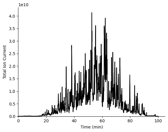
plot_data can be used to plot the TIC and ions per MS1 scan in a pandas DataFrame.
msplot.plot_data(ms1_df)
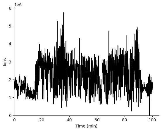
msplot.plot_data(ms1_df, data_type="ions")
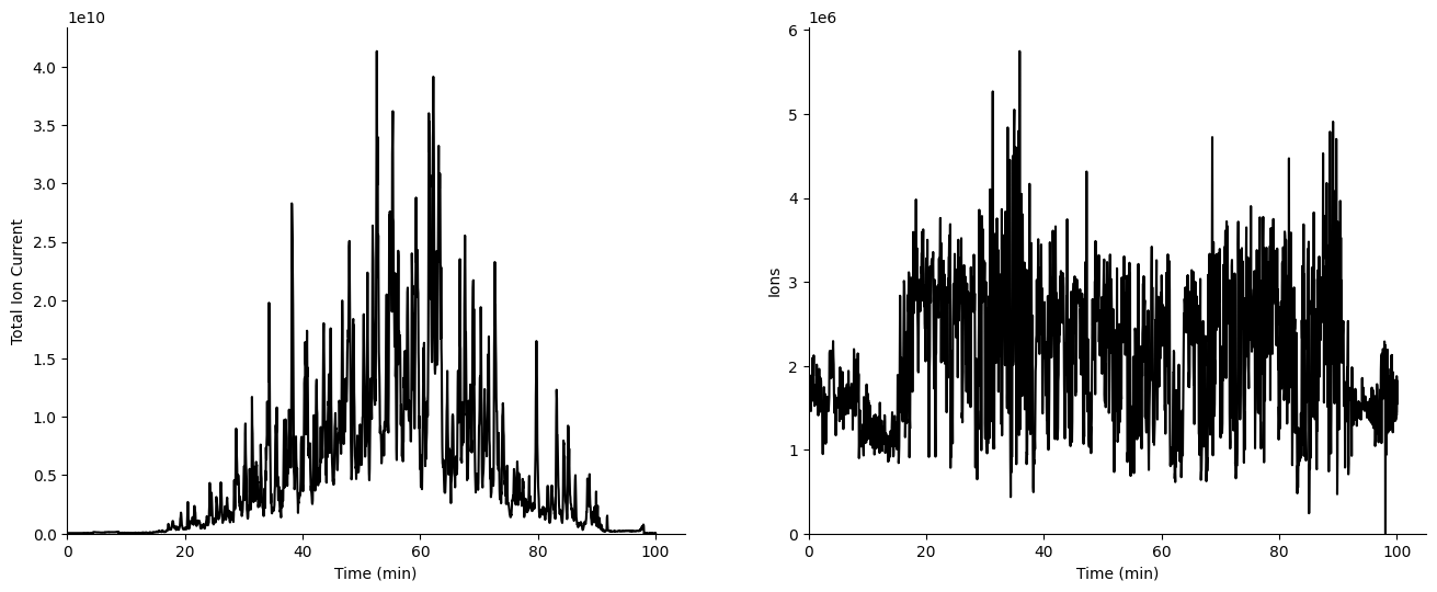
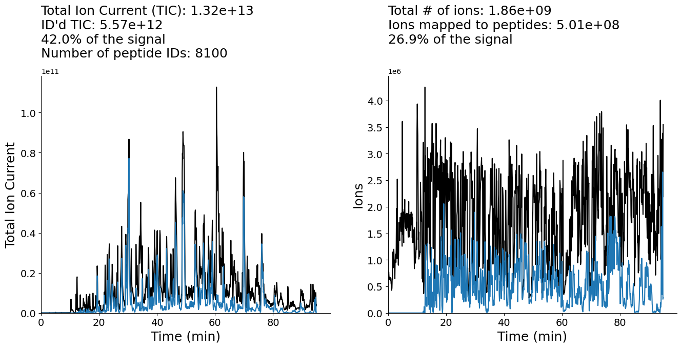
msplot.plot_data(ms1_df, data_type="both")
plot_data can also take mzML files as input.
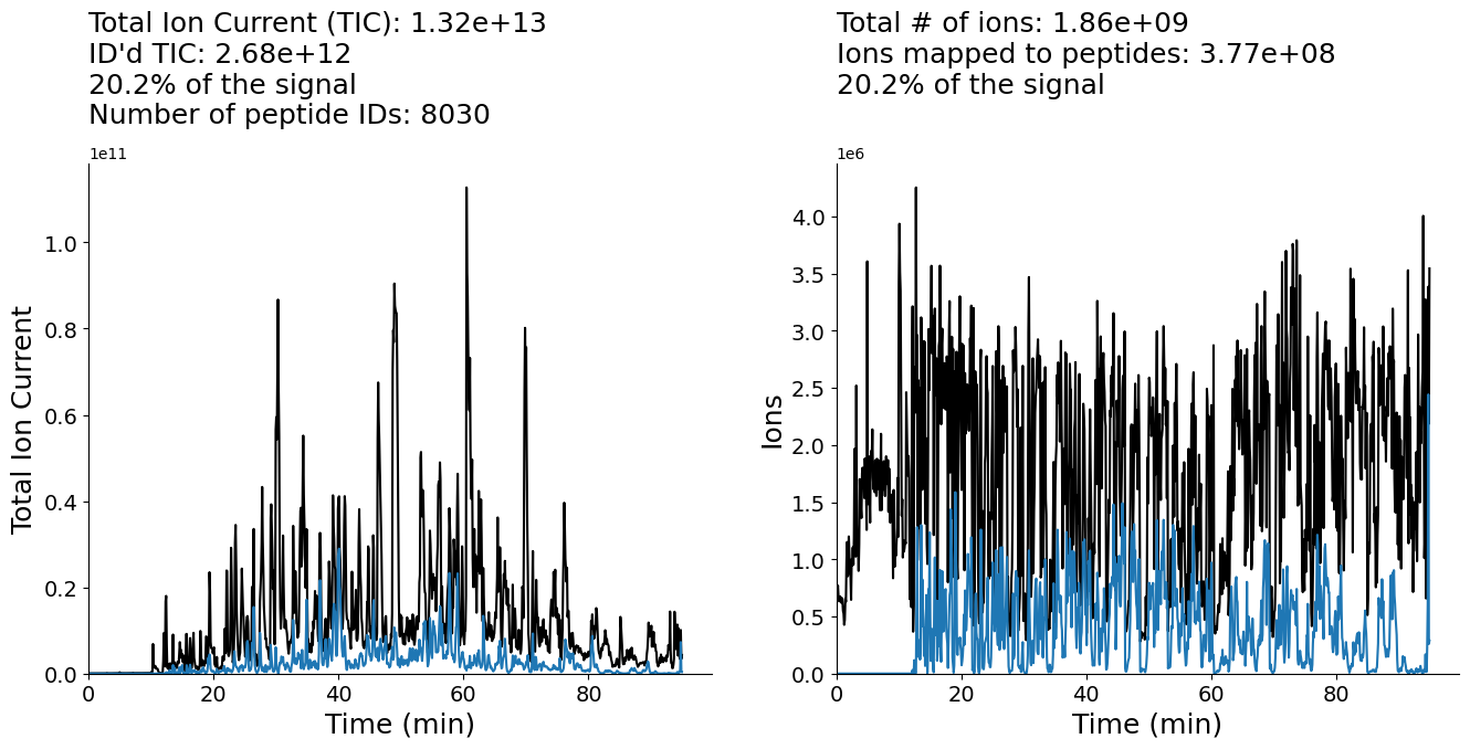
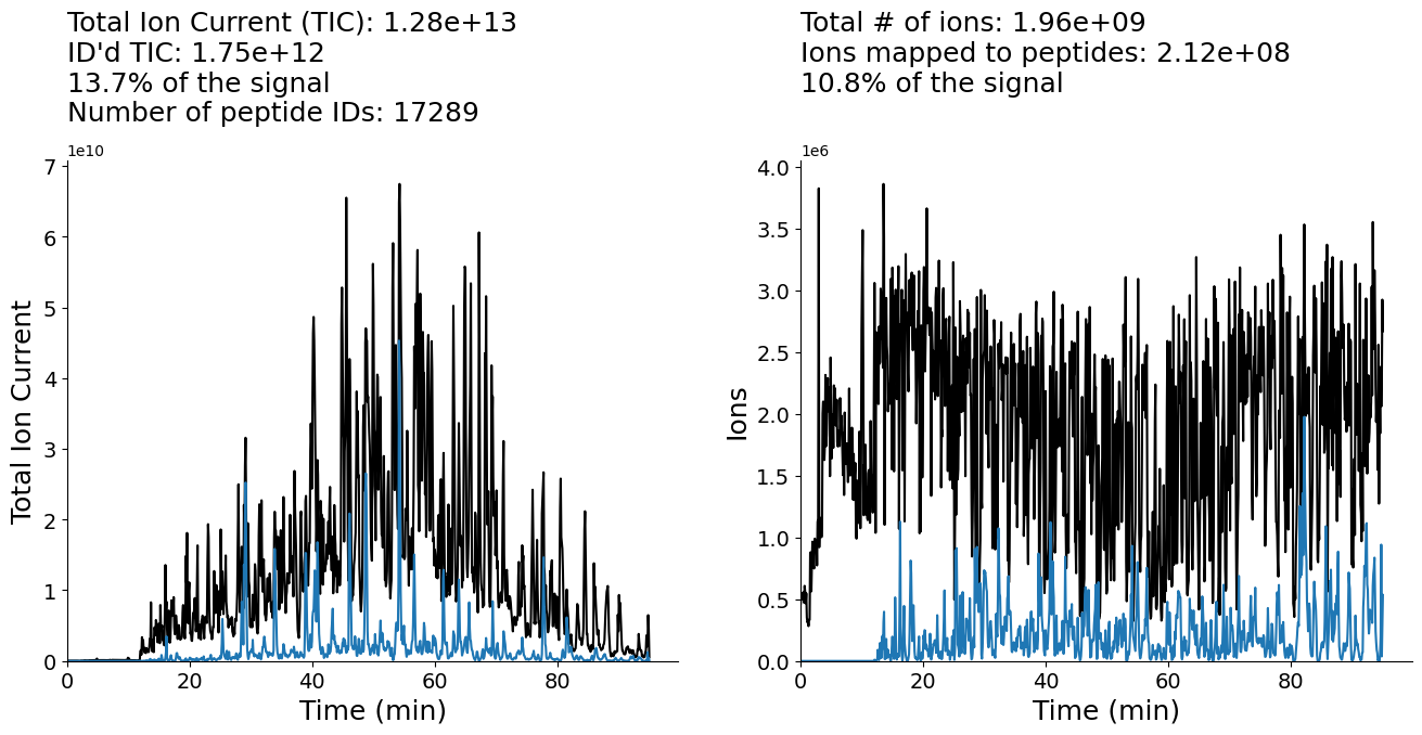
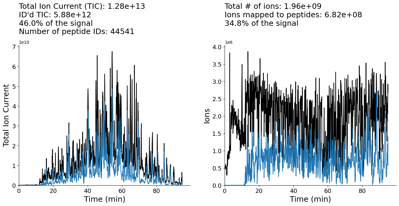
plot the amount of identified signal if you provide a feature file/DataFrame and the identifications file/DataFrame.
Miscellaneous utility functions
bin_list creates a list of bin edges for a histogram.
# define arguments
mz_bin_size = 4
mz_bin_mult = 1.0005
mz_start = 399
mz_end = 1005

bin_mz_list = msutils.bin_list(mz_start, mz_end, mz_bin_size, mz_bin_mult)
bin_data bins a pandas DataFrame using list(s) of bin edges.
msutils.bin_data(ms1_peaks, type="mz", bin_mz_list=bin_mz_list)
| rt | bin_mz | ips | |
|---|---|---|---|
| 0 | 32.542579 | [399.0, 403.002) | 1.048150e+08 |
| 1 | 32.542579 | [403.002, 407.004) | 4.862561e+06 |
| 2 | 32.542579 | [407.004, 411.006) | 5.346059e+06 |
| 3 | 32.542579 | [411.006, 415.008) | 5.346583e+06 |
| 4 | 32.542579 | [415.008, 419.01) | 7.255431e+06 |
| ... | ... | ... | ... |
| 5129 | 33.093167 | [983.292, 987.294) | 2.364387e+06 |
| 5130 | 33.093167 | [987.294, 991.296) | 2.474095e+06 |
| 5131 | 33.093167 | [991.296, 995.298) | 3.682017e+06 |
| 5132 | 33.093167 | [995.298, 999.3) | 3.545738e+06 |
| 5133 | 33.093167 | [999.3, 1003.302) | 4.575072e+06 |
5134 rows × 3 columns
Technical Note Use Cases
# initiate dictionary to store data
note_dict = {}
EV
file_name = "Ecl_2022_0718_FreezeThaw_Q1_EV10_12mz_26"
suf = ""

note_dict[file_name+"_ms1"+suf], note_dict[file_name+"_sumid"+suf], note_dict[file_name+"_id"+suf], note_dict[file_name+"_hk"+suf] = msplot.plot_data(human_dir+"mzMLs/SixQuantitativeIons/"+file_name+".mzML",
                 human_dir+"hk_files/"+file_name+"_MS1_3sn.hk",
                 human_dir+"mzMLs/SixQuantitativeIons/"+file_name+".mzML.elib",
                 method="DIA", data_type="both", stats="title", return_dfs=True)

Plasma
file_name = "Ecl_2022_0718_FreezeThaw_Total_01_12mz_28"
suf = ""

note_dict[file_name+"_ms1"+suf], note_dict[file_name+"_sumid"+suf], note_dict[file_name+"_id"+suf], note_dict[file_name+"_hk"+suf] = msplot.plot_data(human_dir+"mzMLs/SixQuantitativeIons/"+file_name+".mzML",
                 human_dir+"hk_files/"+file_name+"_MS1_3sn.hk",
                 human_dir+"mzMLs/SixQuantitativeIons/"+file_name+".mzML.elib",
                 method="DIA", data_type="both", stats="title", return_dfs=True)
Mouse DB
file_name = "Ecl_2022_0718_FreezeThaw_Q1_EV10_12mz_26"
suf = "_mus"
mzml_dir = "mzMLs/mouse_fasta/"

note_dict[file_name+"_ms1"+suf], note_dict[file_name+"_sumid"+suf], note_dict[file_name+"_id"+suf], note_dict[file_name+"_hk"+suf] = msplot.plot_data(human_dir+mzml_dir+file_name+".mzML",
                 human_dir+"hk_files/"+file_name+"_MS1_3sn.hk",
                 human_dir+mzml_dir+file_name+".mzML.elib",
                 method="DIA", data_type="both", stats="title", return_dfs=True)
Missing Albumin
file_name = "Ecl_2022_0718_FreezeThaw_Q1_EV10_12mz_26"
suf = "_noalbu"
mzml_dir = "mzMLs/SixQuantitativeIons/"

note_dict[file_name+"_ms1"+suf], note_dict[file_name+"_sumid"+suf], note_dict[file_name+"_id"+suf], note_dict[file_name+"_hk"+suf] = msplot.plot_data(human_dir+mzml_dir+file_name+".mzML",
                 human_dir+"hk_files/"+file_name+"_MS1_3sn.hk",
                 human_dir+mzml_dir+file_name+".mzML_noALBU.elib",
                 method="DIA", data_type="both", stats="title", return_dfs=True)
file_name = "Ecl_2022_0718_FreezeThaw_Total_01_12mz_28"
suf = "_noalbu"
mzml_dir = "mzMLs/SixQuantitativeIons/"

note_dict[file_name+"_ms1"+suf], note_dict[file_name+"_sumid"+suf], note_dict[file_name+"_id"+suf], note_dict[file_name+"_hk"+suf] = msplot.plot_data(human_dir+mzml_dir+file_name+".mzML",
                 human_dir+"hk_files/"+file_name+"_MS1_3sn.hk",
                 human_dir+mzml_dir+file_name+".mzML_noALB.elib",
                 method="DIA", data_type="both", stats="title", return_dfs=True)